Project Finance Modelling: Cash Flow Waterfalls, DSCR Sizing and the Debt Sculpt

The structure that dictates the model

A project company is formed to build and operate one asset — a wind farm, a toll road, a hospital, a transmission line. Lenders lend to that entity against its contracted revenues. If the project fails, they take the asset and its contracts; they have no claim on the sponsors beyond their equity.

That makes revenue contract quality the credit. A project with a twenty-year offtake agreement at a fixed price with an investment-grade counterparty supports far more leverage than one selling into a merchant market, because the lender is really underwriting the contract rather than the asset.

It also means the model must run over the full concession or contract life. A five-year forecast is meaningless when the debt tenor is eighteen years and the sculpting depends on cash flows in year fifteen.

Two phases, modelled differently

The construction phase has no revenue and heavy outflows. You model the drawdown schedule against a construction programme, interest during construction (which is capitalised into the project cost rather than expensed), commitment fees on undrawn facilities, and a contingency line that most models under-size.

The operations phase begins at commercial operation date. Revenue follows the offtake contract — availability payments, a power purchase agreement tariff, tolls — with any indexation modelled explicitly. Operating costs split between fixed operations and maintenance, variable costs, and the periodic major maintenance that is a defining feature of infrastructure assets.

The transition between them matters. Delay to commercial operation date pushes revenue back while interest continues to accrue, and modelling a construction delay scenario is standard because it is the risk lenders care most about.

The cash flow waterfall

Cash in a project company is not available to whoever wants it. It moves through a contractually defined order of priority, and modelling that order correctly is most of the work.

The standard sequence: revenue in; operating costs; taxes; senior debt interest; senior debt principal; funding of the debt service reserve account to its required level; funding of the maintenance reserve account; subordinated or shareholder debt service; then, and only if all distribution lock-up tests are met, dividends to equity.

The lock-up test is the mechanism that protects lenders. If the DSCR falls below a defined threshold — commonly 1.10x to 1.20x against a covenant set slightly lower — cash is trapped in the project rather than distributed. Model it as an explicit switch, because a model that distributes cash through a lock-up overstates equity returns and misrepresents the risk.

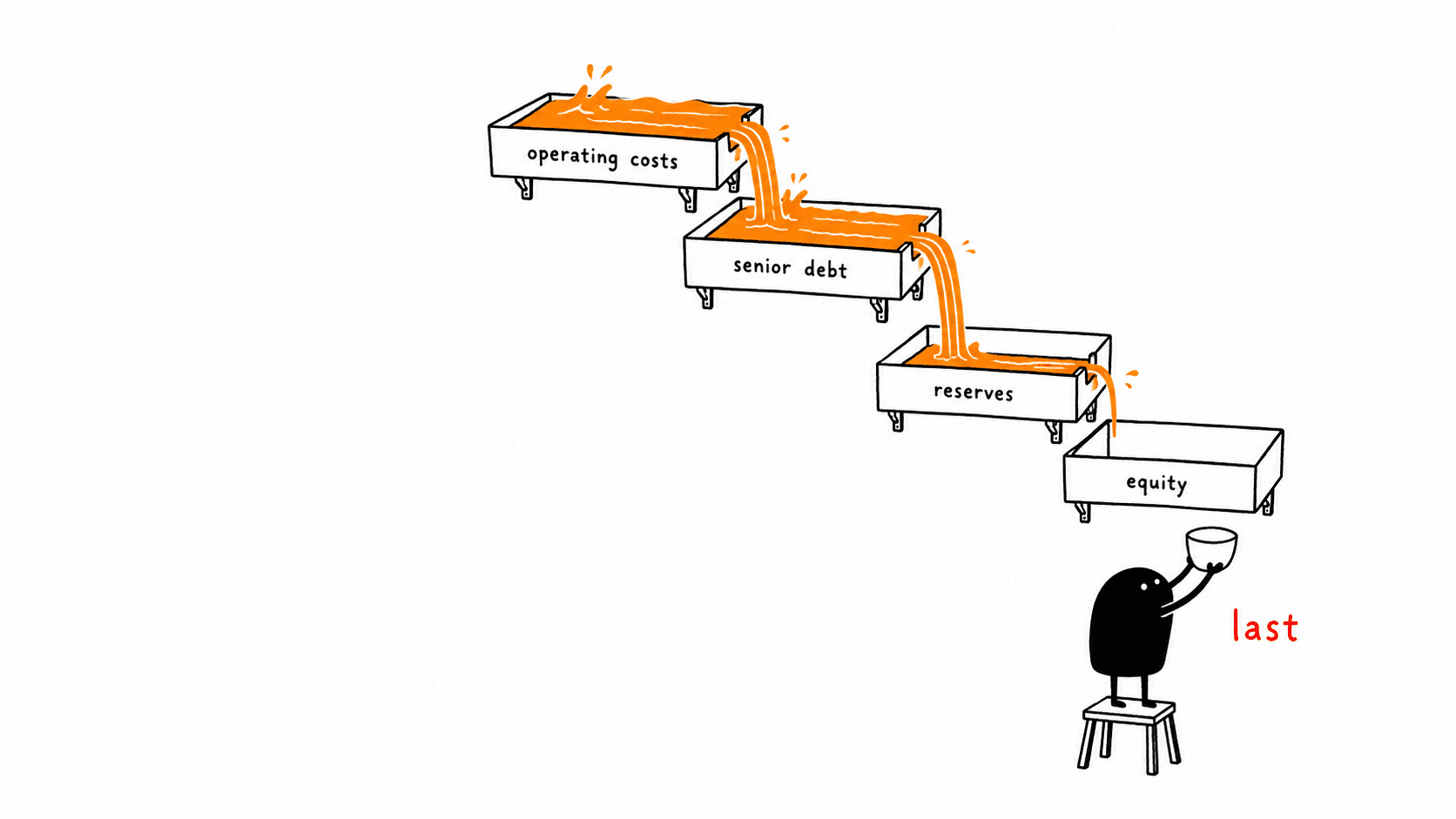
• Operating costs and taxes first.
• Senior interest, then senior principal.
• Debt service reserve account topped to its target, usually six months of debt service.
• Maintenance reserve funded against the major maintenance schedule.
• Subordinated debt.
• Equity distributions, subject to the lock-up DSCR test being met.

Sizing and sculpting the debt

Project finance debt is sized to a target debt service coverage ratio rather than to a leverage multiple. The lender sets a minimum DSCR for the project type — typically around 1.30x to 1.45x for contracted renewables, higher for merchant or demand-risk assets — and the debt is whatever produces that coverage.

Sculpting is the technique that makes this work. Rather than a flat amortisation profile, the repayment schedule is shaped so that debt service in each period equals that period’s cash available for debt service divided by the target DSCR. The result is a profile that repays more in strong years and less in weak ones, maximising debt capacity while holding coverage constant.

Mechanically: calculate cash available for debt service for every period; divide each by the target DSCR to get the affordable debt service; strip out the interest component to get the principal repayment; then discount the repayment schedule back to get the supportable debt quantum. This is circular — interest depends on the balance, the balance depends on repayments, repayments depend on interest — so it is either an iterative calculation or a goal-seek, and it must be flagged as such in the model.

The coverage ratios lenders actually monitor

DSCR is the period test: cash available for debt service divided by debt service in that period. It is calculated for every period and reported as both a minimum and an average across the debt life.

The loan life coverage ratio takes a whole-life view: the net present value of cash available for debt service over the remaining loan term, divided by the outstanding debt balance. Where DSCR can look acceptable in a given period while the project is heading for trouble later, LLCR catches it. Lenders typically want it above 1.4x.

The project life coverage ratio extends the same calculation to the full asset life rather than the debt tenor, capturing the tail value beyond debt maturity — relevant where the concession runs materially longer than the loan.

Where project finance models go wrong

Three failures recur, and all three are structural rather than arithmetic.

Modelling annually. Debt service, reserve accounts and lock-up tests operate quarterly or semi-annually, and an annual model averages away exactly the periods where coverage is tightest. Build at the frequency the debt actually operates at.

Omitting the reserve accounts. The debt service reserve and maintenance reserve consume cash before equity sees any, and a model that ignores them overstates distributions in the early years, which is where the equity IRR is most sensitive.

Treating the lock-up as advisory. If the model distributes cash while the DSCR is below the lock-up threshold, the equity return is fiction. It has to be a hard switch, tested every period.